REDCAT Documentation Table of Contents
Tutorials
Tutorial #1: Synthesizing Data
Starting the program
- Create a working subdirectory. For our example: "mkdir REDCAT_test". This is recommended since REDCAT creates a number of intermediate files that are not always deleted. Therefore it is a good practice to contain these files by putting them in one directory.
- Change the directory to the working directory. "cd REDCAT_test"
- Start the program by typing "REDCAT.tcl" or any other alias name.
Generating an input file
- Here you will need to have a PDB file. Before proceeding, make sure that the PDB file is a well behaved one, and does not contain multiple models. If so, just edit the file and delete all of the models except the working model. This tutorial will utilize the PDB file "1a1z.H.pdb" which is supplied with the package in the REDCAT/data directory. For simplicity, copy this PDB file into your current directory.
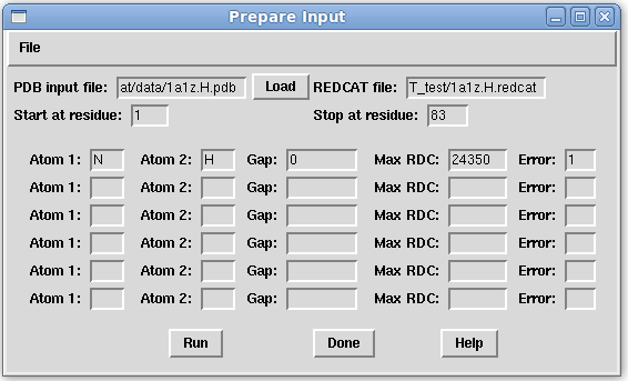
- On the Main window menu bar, click "File:Prepare Input" and complete the form as pictured below. If the PDB file is in the directory that REDCAT was launched from, a complete path is not needed, otherwise please specify the complete path. Click the "Run" button on the Prepare Input window to create the REDCAT file, then close the "Done creating the file..." dialog message by clicking the "OK" button. Now, the REDCAT input file has been created and saved. Close the Prepare Input window by clicking the "Done" button. For more information see the Prepare Input section of the Main Gui page of this website.
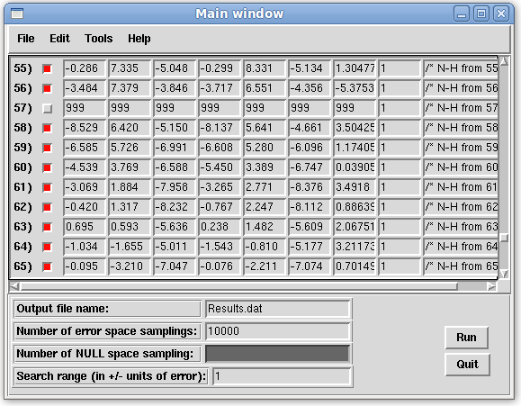
- On the Main window menu bar, click "File:Load:Load Redcat File" and select "1a1z.H.redcat", the REDCAT input file that was created in the previous step. The loaded file should be displayed in the Main window of REDCAT, as shown below.
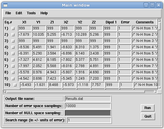
- Note that all of the entries are excluded since they are all missing the RDC values. Also note that the first, third, and fifty-seventh equation entries have repeated coordinates of 999. This is because residue one is has additional hydrogens and residue 3 and 57 are Prolines.
- In order to back calculate these RDC values, first all valid entries must be selected. For our example, we need to select all entries except entry numbers 1, 3, and 57.
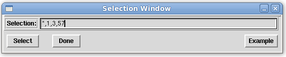
On the Main window menu bar, click on "Edit:Select". In the Selection window that appears, select all entries followed by excluding numbers 1, 3 and 57 (using the expression below) in the text box provided.
*,1,3,57
- Clicking on the "Select" button performs the selection specified in the textbox on of the Selection window.
- Once the proper selections have been made (you can double-check this by scrolling through the Main window and making sure that the checked equation checkboxes match your selections), click "Done" to close the Selection window.
- The "Example" button lists helpful syntax used here.
- For more information see the Selection section of the Main Gui page of this website.
- Next, a diagonal order tensor and Euler angles must be provided so that REDCAT can back-calculate RDC values from the loaded atomic coordinates and this tensor. On the Main window menu bar, click on "Tools:Calculations:Calculate/Substitute RDC" and complete the following fields (Sxx, Syy, Szz, a, b, and c) by typing in the values shown below.
Sxx: 2e-4 Syy: 5e-4 Szz: -7e-4
a: -40 b: -50 c: 60
- Another example of a possible order tensor (not used in this tutorial) is listed below:
- Note, Sxx + Syy + Szz = 0. An error will be received if this is not true.
An example input value not used here:
Sxx: -3e-4 Syy: -5e-4 Szz: 8e-4
a: 0 b: 0 c: 0
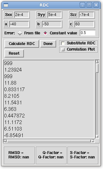
- Note that, in the above RDC window, the "Substitute RDC" button has been checked. This will substitute the calculated RDC values in the loaded input file.
- Also note that the "Constant value" radio button has been selected and that a value of 0.5 has been entered in the corresponiding textbox. This simulates adding random experimental error between -0.5 Hz and 0.5 Hz. While not used in this tutorial, error can also be added by taking the error associated with each equation (listed under the error column in the Main window) by instead selecting the "From file" radio button.
- Once all the fields in the RDC winodw have been addressed, continue by clicking the "Calculate RDC" button. This will back-calculate the RDC values. On the Main window, the RDC values for the selected equations will have changed.
- Close this window by clicking "Done".
Data Analysis
- Engage the analysis engine by clicking on “Run” in the Main window.
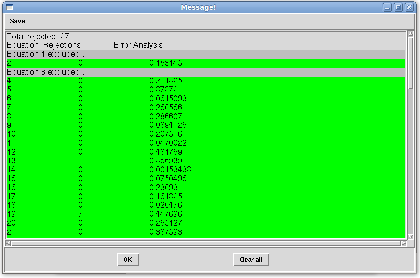
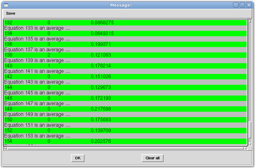
- The “Message!” window should appear after a few seconds (depending on the computational resources available) with the analysis status. The analysis should appear similar to the following below. You should have very small number of rejections since the data was generated with error of 0.5 Hz and allowed error was 1.0 Hz.
- To observe the solutions, on the Main window menu bar click on “Tools:Solution:Get Solutions”. The solutions will be appended to the bottom of the "Message!" window following the error analysis results generated in the previous step. To see the solutions at the top of the "Message!" window, the contents of the “Message!” window can be cleared by using the “Clear all” button prior to clicking on "Tools:Solution:Get Solutions". The contents of the "Message!" window can be saved at any time by using the save menu option in this window. Once the solutions are obtained, any one of the resulting solutions can be selected in order to back calculate RDCs and confirm correct function. The RMSD value reported by the “Calculate/Substitute RDC” tool can also be used to confirm that the best solution results in the best RMSD value. In doing so, make sure that the "Substitute RDC" check box is not checked. For more information see the Message section of the Main Gui page of this website.
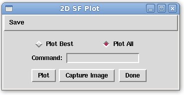
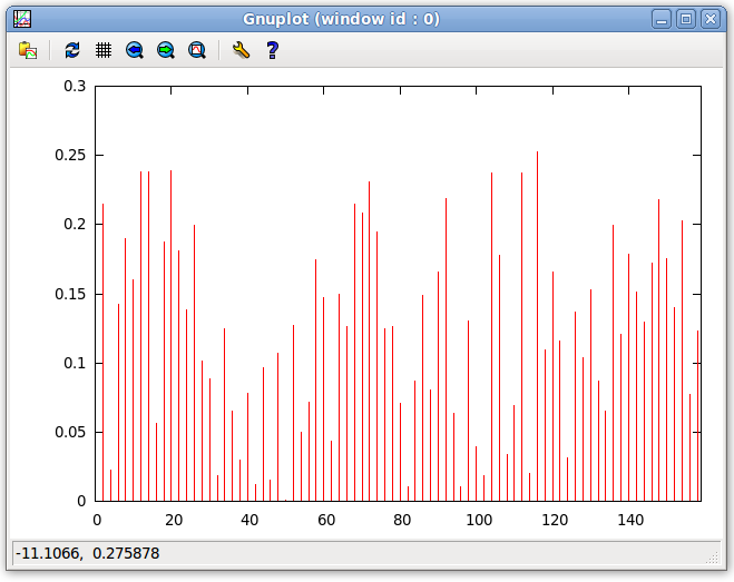
- For visual inspection of the PAF within the molecular frame, on the Main window menu bar click on “Tools:Plot:2D SF Plot”. The 2D SF Plot window shown below will appear. Select "Plot All". Clicking on the "Plot" button will generate a gnuplot window similar to the graph below. If the program returns an error message related to “map.out”, make sure that the 2D map location is set correctly; this can be changed by navigation to the Main window bar and clicking on "Edit:Options". For more information see the SF Plot section of the Main Gui page of this website.
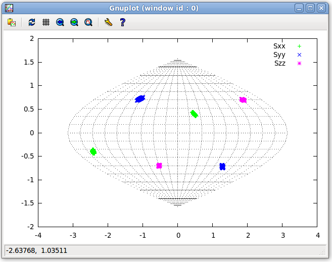
- Note, for those not familiar with gnuplot, the numbers in the bar immediately below the plot correspond to the mouse's position on the plot and, for the purpose of these tutorials, are not important.
Saving the input file for Tutorial 2
- On the Main window menu bar, click on "File:Save:Save Redcat File" and save this file for use with other tutorials. For simplicity, you can name this file Tut_one.redcat.
Tutorial #2: Error Analysis
Generating Error Analysis
Here, you will learn how to perform error anlysis with REDCAT. Please, load the file created at the end of the previous Tutorial, or continue on from Tutorial 1.- On the Main window menu bar, click on "Tools:Error Analysis:Perform Error Analysis" to bring up the "Message!" window. This window will show the Rejections and Error for each equation. The Rejection section corresponds to the number of times the specific equation contributed to the rejection of a Monte Carlo sample. The Error section shows the error between the back-calculated RDC and the provided RDC values. In the previous version of REDCAT, Monte Carlo rejection analysis and error analysis were separate features. Now, we have tied these two features together, to facilitate ease-of-use and allow for faster analysis. In our example, the Rejections will be very low as the random error we have added is only 0.5 Hz. The Error, as well, will be below 1 Hz for each equation. For more information see the Message section of the Main Gui page, or the Viewing and Interpreting Results page of this website.
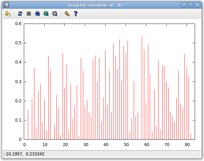
- On the Main window menu bar, click on "Plot:Plot Violations". This will generate a gnuplot of the Error for each equation. This plots the error of each equation as a bar chart. Using this plot, the user can see which points are in violation. This plot is also useful for finding outliers that may correspond to misassigned data. For more information about the plot below, see the Viewing and Interpreting Results page of this website.
- On the Main window menu bar, click on "Tools:Solution:Get Solutions". In the "Message!" window, the least squares solution (Tensor 0), as well as many more Tensors, which represent the Monte Carlo solution that did not fall beyond the error specified, are seen. Depending on the quality of the loaded RDC data, the number of order tensors produced should vary between one and the number of Monte Carlo samples specified can be viewed here. These order tensors are appended to the bottom of the "Message!" window, so if you do not see them right away, scroll down throught the display window. Select the radio button next to Tensor 0 as shown below.
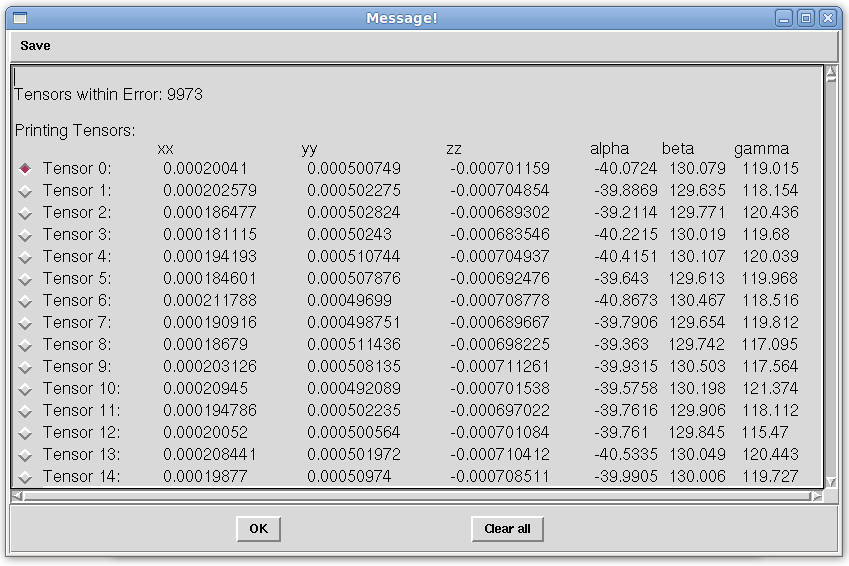
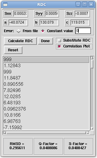
- Once Tensor 0 is selected, the principal order parameters (Sxx, Syy, and Szz) and Euler rotations (&alpha, &beta, and &gamma) are loaded into various windows which require these parameters. On the Main window menu bar, click on "Tools:Calculations:Calculate/Substitute RDC". This brings up the RDC window. The principal order parameters as well as the Euler rotation angles will already be loaded. Select the "Constant value" radio button and in the entry box next to it, enter the value 0. Here we state that we would like to add random error of zero to each back-calculated RDC value. If the "From file" radio button were to be selected instead, random amounts of error varying from zerio to the number specified in the Main window, would be added to each RDC equation. In our example, this would add a random number between zero and the one for each RDC. Select the "Correlation Plot" checkbox, as in the picture below, -- if you continued on from Tutorial 1 please ensure the "Substitute RDC" check box is not selected -- and then click the "Calculate RDC" button. This will create a correlation plot, similar to the graph below, that plots the back-calculated (Computed) RDC value vs. the provided (Measured) RDC value. The RMSD, Q-Factor, and S-Factor is given at the bottom of the window RDC window. The closer the RMSD value is to zero, the better the fitness of the back-calculated RDC values is to the provided RDC values. The closer the Q-Factor and S-Factor is to zero, the less noise there is in the back-calculated RDCs and provided RDCs, respectively.
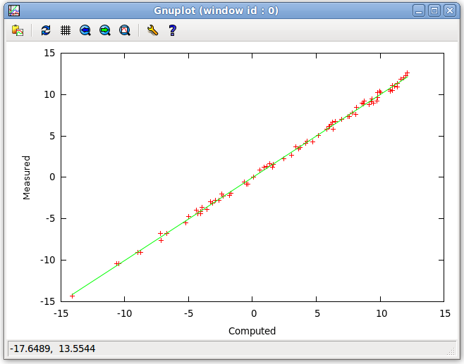
- The Correlation Plot exemplified below, shows the user the R2 regression line and plots the Computed RDC vs. the Measured RDC as described above. This allows the user to see the fitness of the back-calculated RDC values to the provided RDC values. Here outliers can be seen which may help to identify misassignment.
Tutorial #3: Dynamics Part I: Emulation
The Dynamic Averaging feature of REDCAT allows a user to average n states of RDCs over a dynamic domain. This is done by applying a rotation for each state to the selected domain, and back-calculating RDCs for that rotation. These back-calculated RDCs are then averaged, using their probability as weight in averaging, and the average is then substituted for each RDC selected.
C3 Molecular Symmetry
Please close any loaded data and open the file generated in Tutorial 1. If you have not completed Tutorial 1, please do so before continuing. For Tutorial 1, please click the following link. Tutorial #1: Synthesizing Data
- After ensuring that the correct file is loaded, in the Main window menu bar click on "Edit:Select". In the Selection window, select all values with loaded data using the expression below.
*,1,3,57
- In the Main window menu bar, click on "Tools:Calculations:Dynamic Averaging". This opens the Dynamic Averaging window, pictured below. Input the currently loaded REDCAT file as the input file. Specify the output file as 1a1z.AVG.redcat. Next, load the states.in file from the data subdirectory under the Redcat installation directory. You will need to provide the full path to this file, or copy it from the data directory under the install directory, to the REDCAT_test directory. The states.in file contains 3 states specified here. Next, generate Tensors as done in Tutorial 2. Please click the "Run" button on the Main window. From the Main window menu bar, click on "Solutions:Get Solutions". Finally, scroll down to Tensor 0 on the "Message!" window and select the radio button to its left to populate the Sxx, Syy and Szz portions of the Dynamic Averaging window. Click the "Average" button on the Dynamic Averaging window. This will apply the dynamic averaging to the selected equations on the Main window. In this case, all equations are averaged.
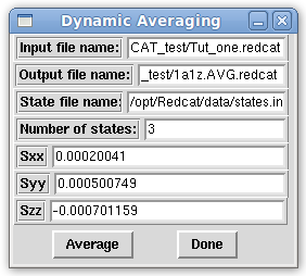
- On the Main window, the RDC values for the selected equations will have changed. The output file specified in the Dynamic Averaging window will reflect the same information seen below.
More information about the states.in file can be found on the Dynamic Averaging File Format section of the File Formats page this website. For more information about the Dynamic Averaging window, please refer to the Dynamic Averaging section of the Main Gui page on this website.
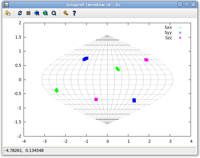
- The effects of this type of dynamic is predictable. It can be analytically shown that this type of symmetry will result in an axial symmetry. As the new data has not yet been run, REDCAT still has stored within it the data from before dynamic averaging was performed, even though the Main window will show some equations not related to the previous run. This information will not be updated until the "Run" button on the Main window is clicked again. Before a new run is performed on the dynamically averaged data, look at the plot of the previous Tensor to compare with the Tensor of the dynamically averaged data. On the Main window menu bar, click on "Tools:Plot:2D SF Plot". Select the "Plot all" radio button on the 2D SF Plot window and click on the "Plot" button. This will result in the plot seen below.
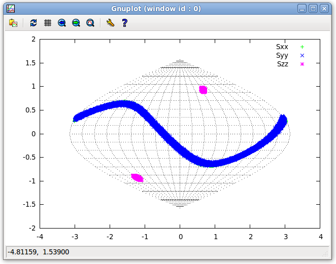
- Now, look at the Plot from the dynamically averaged data. Click the "Clear All" button on the "Message!" window. Click on the "Run" button on the Main window, then on the Main window menu bar click on "Tools:Solutions:Get Solutions" and scroll to Tensor 0. Select the radio button to its left to replace the old tensor information with the new tensor derived from the dynamically averaged data. Going back to the 2D SF Plot window, clicking on the "Plot" button will produce the image below.
Emulating Internal Motion at the Terminal Helix of 1A1Z
For this illustration, we will synthesize data for 1A1Z and emulate the effects of a certain hypothetical dynamic on the terminal helix of this structure. Analysis of the data will follow after the synthesis. Please close any loaded data and open the file generated in Tutorial 1. If you have not completed Tutorial 1, please do so before continuing.
- Create the states file as shown below and save it as states.in under the REDCAT_test directory created from Tutorial 1. For more information about the states file format, please see The Dynamic Averaging File Format page of this website.
0 1.141 -0.571 -0.927 0   0.5
0 1.141 -0.571 -0.927 120 0.5
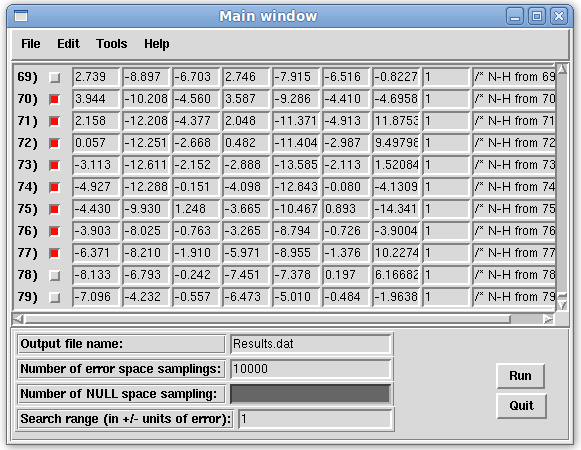
- Select entries 70-77 (residues 73-80) by first excluding them and then negating your selection with the following statement in the "selection" box. Here, the equations that correspond to the terminal helix are selected. The RDC value of these equations will change to simulate the two state motion.
*,!,70-77
Below is an example demonstrating the Main window after this step.
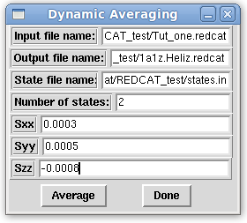
- Open the Dynamic Averaging window by selecting from the Main window menu bar "Tools:Calculations:DynamicAveraging." Place the Tut_one.redcat file as the input file, and 1a1z.Helix.redcat as the output. Use the states file created above. Use 0.0002 for Sxx, 0.0005, for Syy, and -0.0007 for Szz. These are the ideal values used to generate the data in Tutorial 1. Click on "Average" to modify the RDC values of residues 70 to 77 to simulate motion described in the user created states.in file.
- Now, we must select all equations in order to see the run the dynamically averaged portion and compare the error of residues 70-77 to the rest of the structure. Open the Selection window by clicking on "Edit:Select" on the menu bar of the Main window. Select all equations with complete data by entering the following in to the Selection window and clicking the "Select" button.
*,~
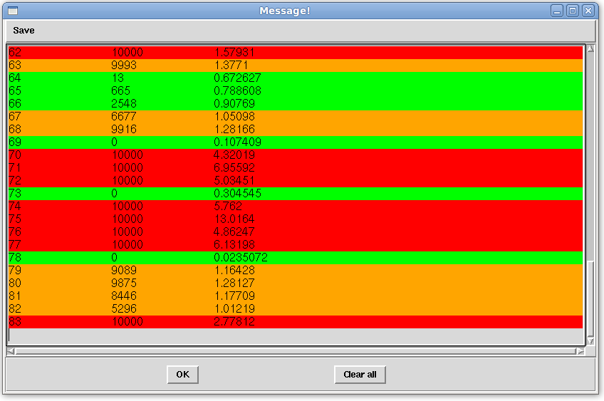
- Click the "Run" button on the Main window to perform analysis on all equations to see the outcome of the dynamic averaging of the terminal Helix. The error analysis will be displayed in the "Message!" window as shown below, and should be similar.
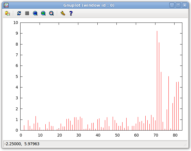
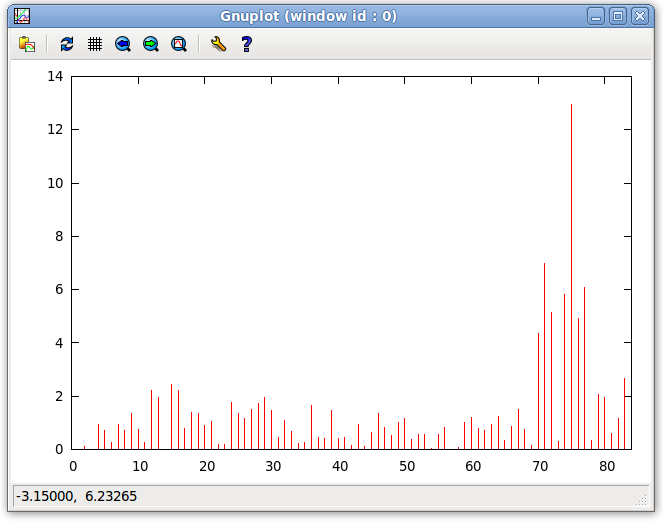
- The errors displayed in the previous step can be plotted as a function of the entry number by clicking "Tools:Plot:Plot Violations" on the menu bar of the Main window. This plot is shown below. As seen in the plot below, equations 70 to 77 have high error terms indicating that the simulated movement does not correspond to the given structure. Under a structure which does undergo internal dynamics, without Dynamic Averaging the structure would show high error, however, with correct internal dynamics, the error for the dynamic regions would lower.
Tutorial #4: Dynamics Part II: "AVG" Directive
As illustrated during Tutorial 3, REDCAT is capable of calculating the effects of dynamics on RDC data. This information is useful to confirm or reject proposed dynamical regions. However, when the nature of the motion is known, it appears that we should be able to integrate the RDC data from the motional regions as well as the static regions. This objective can be achieved by using the "AVG" directive. This directive can be used in a variety of situations that may not include any motion. For example, one can use this directive in including the RDC collected from aromatic side chains with documented 180° flips, to include the combined RDC data from both Ha protons of Glycines and chemical shifts changes.
In this tutorial, we will model the motion of the terminal helix that was simulated in Tutorial 3. By modifying the ψ angle of residue 70 of 1A1Z by 180°, we reorient its terminal helix. A REDCAT file is then prepared from the modified 1A1Z, in the same manor as discussed in Tutorial 1, using the principal order parameters, Euler angles, and constant error value listed below.
Sxx: 2e-4 Syy: 5e-4 Szz: -7e-4
a: -40 b: -50 c: 60
Constant value: 0.5
We provide this file here: 1a1z.M.redcat.
- First, we must create the file containing the AVG RDC values. Manually interlace Tut_one.redcat, created by performing Tutorial 1 (if you have not yet performed Tutorial 1, please do so now by navigating to the Tutorial 1 section of this website.), with 1a1z.M.redcat in such a way that equation one from Tut_one.redcat is the first line of the interlaced file, followed by equation one from 1a1z.M.redcat, followed by equation 2 from Tut_one.redcat, followed by equation 2 from 1a1z.M.redcat, and so on in this fashion. For each equation, take the average of the two RDC values located in column 7, place AVG in the RDC position of the first line, and replace RDC position in the second line with the averaged RDC value. Save this manually interlaced file as Tut_four.redcat. A portion of the prepared file is shown below, for comparison to your manually created file.

- Note, in this example we use only the N-H RDC vector. For more RDC vectors, keep the RDC schema the same for generation of both files. Each vector type for each residue should be kept together when interlacing.
- Load Tut_four.redcat from the Main window menu bar by clicking on the "File:Load:Load Redcat File" and selecting the correct file. Click on the "Run" button on the Main window and observe the results displayed. They will look similar to the results shown below.
- Plot the error by selecting in the Main window menu bar "Tools:Plot:Plot Violations". The bar plot will look similar to the one shown below. Notice that the x axis lists double the number of equations as there were in Tut_one.redcat. This is because half are from Tut_one.redcat and half are from 1a1z.M.redcat. If we count the number of bars between 0 and 20, we see there are only ten. The averaged equations are combined to form a single equation and the evaluation of the averaged equation is shown here. For this reason, only every other equation is listed in the bar graph, leaving extra white space between each datum. Also, note that the error is below the 0.5 Hz noise randomly generated for both sets of data. This shows that the analysis illustrates the motion well.
- We would like to see what happens when we look at the averaged RDCs that describe the motion of the terminal helix and apply them to the static structure. To do this we must manually create a new REDCAT file that shows one of the two states of the helix and has the RDCs from the averaged structure. Take all RDC values that are not AVG and manually substitute them for the corresponding residues in Tut_one.redcat, and save this new manually created file as Tut_four_error.redcat.
- Close the currently loaded data by clicking in the Main window menu bar "File:Close".
- Load Tut_four_error.redcat by clicking in the Main window menu bar "File:Load:Load Redcat File" and selecting the newly created file.
- Now, we will plot the error in order to compare it with the previous Violation Plot. Run the data by clicking the "Run" button on the Main window. Click on "Tools:Plot:Plot Violations" in the Main window menu bar. The corresponding plot will look very similar to the one below. When we obtain RDC data for regions that undergo motion, we see that the RDC data does not fit the static structure well. This plot, however, is more similar to the plot created in the Internal Motion section of Tutorial 3. In that example, we emulate motion and apply to a static structure. Here we do the same through other means. In both scenarios, the portion of the molecule that undergoes motion has very high error when the motion is applied to a static structure.