


REDCAT Documentation Table of Contents
The REDCAT GUI
Main Window
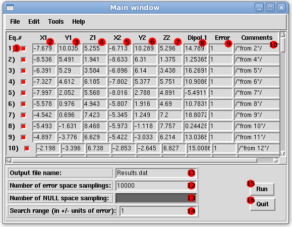
The Main window of REDCAT displays the data associated with the analysis of RDC vectors. The window is broken down into three areas, the menu bar, equation display area, and control panel. Once a REDCAT file is loaded, the display area is populated by the data from the file. A selection box (1) is provided for each equation allowing the user to toggle the inclusion or exclusion of the line in analysis. Each line is broken up into 9 sections: the x (2), y (3), and z (4) coordinates for the first atom, the x (5), y (6) and z (7) coordinates for the second atom, the RDC data for the two atoms (8), the error in Hz associated with the RDC data (9), and a comment about the line (10). These can be modified in line or manipulated by other functions of the program. The "Output file name" entry box (11) specifies the name of the text file generated by the save feature of the "Message!" window. The number of Monte Carlo samples taken from each run can be specified in the next entry box (12). Unfortunately, NULL space sampling (13) has been disabled for the current version of REDCAT. The range of error search can be specified (14). Clicking the Run button (15) will bring up the "Message!" window and populate it with Monte Carlo Rejection and RDC Error Analysis. The Quit button (16) will exit the program. For more information about the menu bar of the Main window, see the Menu Items page of this website.
Message
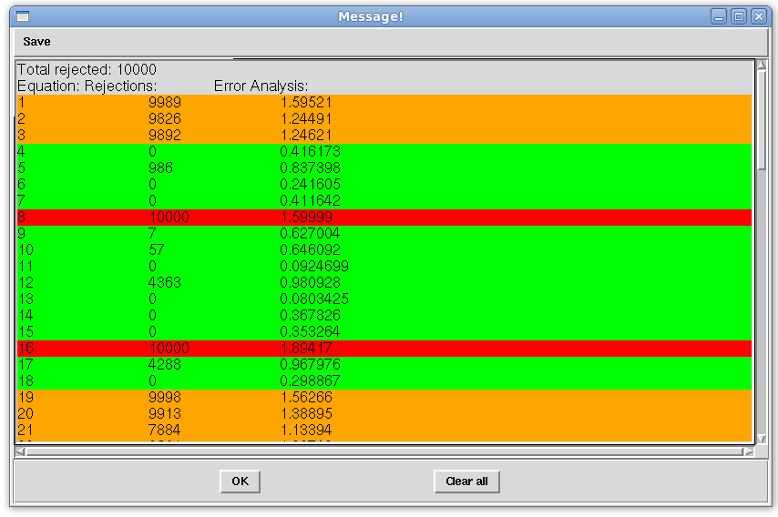
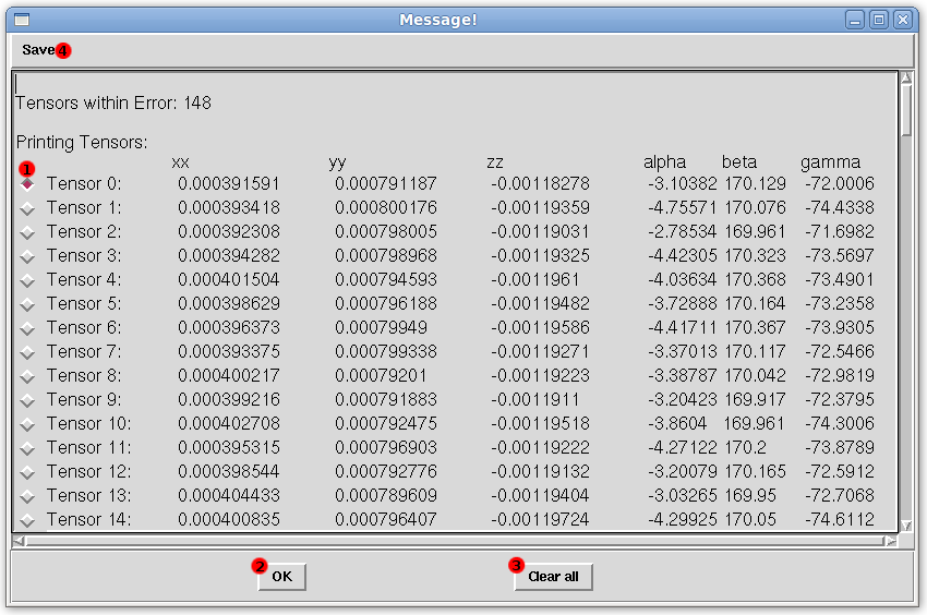
The "Message!" window displays information calculated from the data loaded into REDCAT. Data from multiple REDCAT features is displayed here. All data is added to the bottom of the list until the "Clear all" button is clicked. It is here that users can view data from the current Run, as well as Solutions, and Ensemble structure analysis. When solutions are presented, a radio button is placed beside each Tensor (1). Selecting the radio button loads this data into any window that may take in a tensor and/or rotation.
The window has only two buttons. The "OK" button (2) hides the window, and the "Clear all" button (3) clears the screen of any presented data. The Save menu item (4) can be used to create a text document containing the data currently viewable in the "Message!" window. For more information, please refer to the Viewing Results page of this website.
Prepare Input
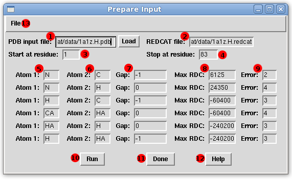
The Prepare Input window is where PDB files are read in and a REDCAT data is created. First, a PDB input file is loaded (1). Next, a name is specified for the REDCAT file that is to be created (2). Starting (3) and ending (4) residues for the protein are specified. These are the residues of interest for RDC analysis in the protein and must be a contiguous portion of the protein.
Next, the RDC criteria is specified. This data includes the two atoms, their relative position to each other, the Dmax associated with the atom pair, and the Error in Hz associated with the RDC type. As shown in the first RDC type in the image above, the atoms, N (5) and C (6) are specified. Since we are concerned with the N of the current residue and the C of the previous residue, a gap distance (7) of -1 is specified. The Dmax (8) associated with the N-C RDC type is used, and an error value of 2 Hz (9) is input. REDCAT can support up to six RDC types in a single file. Each type is specified on a line. For less than 6 RDC types, please start at the top line, and specify each RDC type on the line directly below the previous RDC type. Do not leave any blank lines between RDC types in the Prepare Input window. Once the form is filled out, clicking the "Run" button (10) will process the PDB file and create the REDCAT file.
Clicking the "Done" button (11) will hide the screen, and clicking the "Help" button (12) will display a list of Dmax values for common RDC types that can be used in the "Max RDC" entry box (8). The File menu (13) will open two options, Load and Save. Load will allow you to load a schema file that will populate entry boxes 5-9 for each row. Save will create a schema file from the currently populated entry boxes 5-9 of each row.
Selection
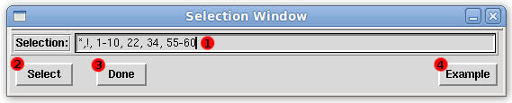
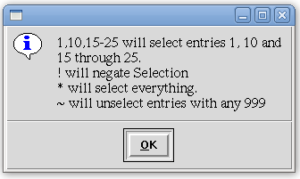
The Selection window allows the user to quickly select and/or omit equations for analysis. The "Selection" entry box (1) allows a user to input a selection statement that will be used to manipulate the equations in the currently loaded REDCAT data file. The pictured example reads as follows. Select all equations, turn them off, select only equations 1 through 10, 22, 34, and 55 through 60. Hitting the enter key while this entry box is active or clicking the "Select" button (2) will execute the selection statement. The "Done" button (3) will hide the window. If additional information about the selection syntax is needed, clicking the "Example" button (4) will show the dialog box pictured below.
Options
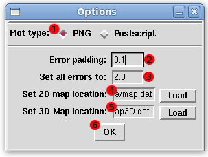
The Options window allows users to specify certain behaviors of REDCAT. The type of image that is plotted can be specified in the plot type section (1). An error pad may be specified (2) and the user may change all errors (3)in the loaded REDCAT file. Maps for 2D (4) and 3D (5) SF plot may be specified. These maps are used to plot selected order tensors. By default the included SF plot maps are loaded. Clicking the "OK" button (6) applies the current entered settings.
Full Report
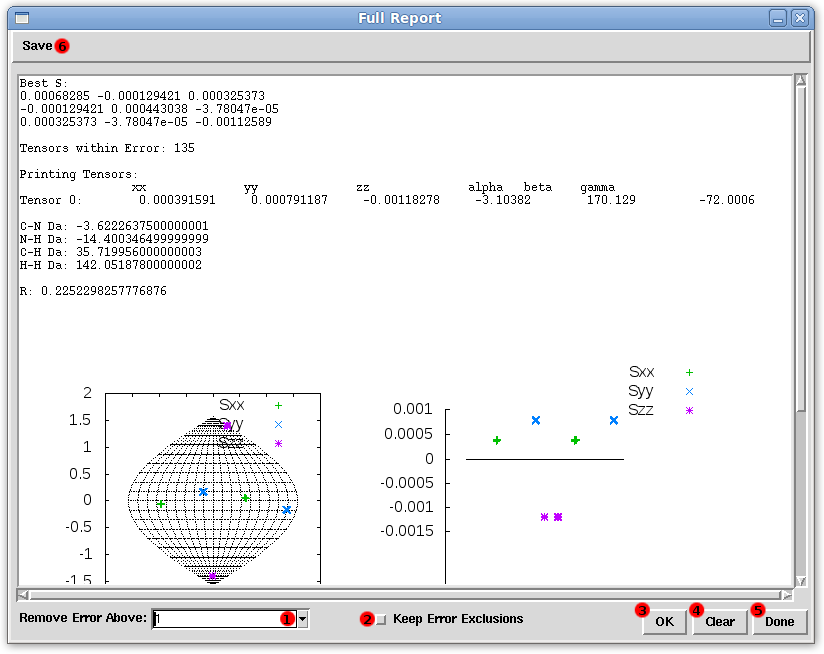
The Full Report window offers the majority of features of REDCAT in a single window. The maximum error in Hz (1) - equations beyond which are filtered out - is specified either by a drop down menu or through manual entry. If the user would like to omit the same equation(s) previously excluded in the Main window, the "Keep Error Exclusions" checkbox (2) should be selected. Clicking the "OK" button (3) will perform the analysis. After performing the analysis, the following information is displayed: the Saupe order tensor matrix; the least squares tensor; Da for the four common RDC types; R; 2D and 3D SF plots; an Error Violation Plot for all equations which fall below the maximum error; and a list of all excluded equations and their error values. Additional analysis will be appended to the bottom of the display. Clicking the "Clear" button (4) will clear all data from the display. Clicking on the "Done" button (5) will hide the window. The Save menu item (6) will save a copy of all text presented on the current display.
Ensemble Solutions
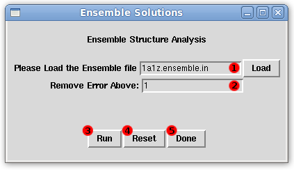
The Ensemble Solutions window can perform quick analysis on multiple REDCAT files and display this side-by-side. This is the same analysis performed by the Full Report window but done for multiple structures. An ensemble file is loaded (1) (For more information about the ensemble file, please refer to the Ensemble Solutions File Format section of this website) and the maximum error in Hz (2) is specified. The "Run" button (3) will perform the analysis and present the data in the Message window. The "Reset" button (4) clears the two entry boxes in the Ensemble Solutions window. The "Done" button (5) hides the window.
2D/3D SF Plot
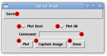
The 2D and 3D SF Plot windows allow the user to visualize the selected order tensor on a Sanson-Flamsteed projection. The plotting of either the least squares order tensor (1) or all proposed solutions (2) can be selected. Commands may be sent in directly to modify the plot via the "Command" entry box (3). The "Plot" button (4) displays the plot. Clicking the "Capture Image" button (5) saves an image of the plot. Clicking the "Done" button (6) hides the window. The Save menu item (7) allows the user to save the raw data points used in the plot. The 3D SF Plot window works the same, with the only difference being that a third dimension corresponding to the value of order parameter being plotted.
Plot Vectors
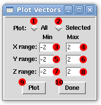
The Plot Vectors window allows a user to visualize all RDC vectors loaded into REDCAT. The user may plot either all vectors (1) or only vectors that correspond to selected equations (2). The minimum (3, 5, 7) and maximum (4, 6, 8) values for the x-axis, y-axis, and z-axis may be specified. The "Plot" button (9) creates a plot containing each vector in blue and the axis system in green. The "Done" button (10) hides the window.
Plot Violations
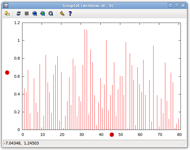
The Plot Violations window is a gnuplot of the Error in Hz (1) of each equation (2). This can be used to obtain an understanding as to the fitness of the data to the structure, as well as to find outliers in the data.
Rotate PDB
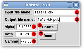
The Rotate PDB window allows the user to create a PDB file with the same structure as a given PDB file with coordinates rotated using an Euler rotation about Z-Y-Z. A PDB file containing the structure of interest is given (1) and the name of the output PDB file is specified (2). The alpha (3), beta (4), and gamma (5) angles are entered. These are populated automatically by selecting a solution in the Message window. The "Rotate" button (6) creates the output PDB rotated by the input information. The "Done" button (7) hides the window.
Rotate Coordinates
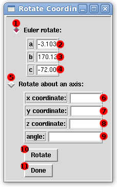
The Rotate Coordinates window rotates the currently loaded coordinates by either an Euler rotation about Z-Y-Z, or about a specified axis by a specified angle. Selection of the "Euler rotate" checkbox (1) will perform the Euler rotation about Z-Y-Z, where a (2), b (3), and c (4) entry boxes correspond to the &alpha, &beta, and &gamma angles. The "a", "b", and "c" entry boxes are populated automatically by selecting a solution in the Message window. While selection of the "Rotate about an axis" checkbox will, instead, rotate about the axis specified by the vector created from the origin to the coordinates specified in the "x", "y", and "z" coordinate entry boxes (6, 7, 8). The coordinates will then be rotated about the specified axis by the angle entered in the "Angle" entry box (9). The "Rotate" button (10) will perform this rotation and the "Done" button (11) will hide this box.
RDC
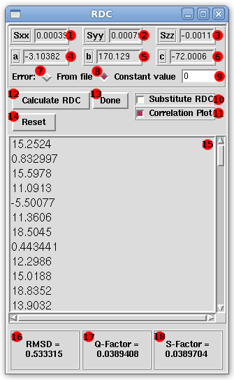
The RDC window allows back-calculation of RDC vectors from the loaded structure, provided an order tensor and a rotation. The principal order parameters may be loaded into the "Sxx" (1), "Syy" (2) and "Szz" (3) entry boxes. The "a" (4), "b" (5), and "c" (6) entry boxes correspond to the &alpha, &beta, and &gamma angles used in the rotation. The principal order parameters and Euler angles are loaded automatically when a solution is selected from the Message window. Random noise can be introduced into the back-calculated tensor. By selecting the "From file" radio button (7), the user specifies that for each equation, the random noise will come from the error specified in the Main window for that equation. The user may instead select the "Constant value" radio button (8); In this case a random noise value can be specified (9) that will be applied to all equations during back-calculation. In the pictured example, there is a random noise of 0 associated with all equations so that no random noise will be generated. If the user would like to replace the RDC data for selected equations in the Main window, they may select the "Substitute RDC" checkbox (10). If the "Correlation Plot" checkbox (11) is selected the back-calculated RDC (labeled Computed) will be plotted against the provided RDC (labeled Measured). An R2 regression line will be applied to the plot. Clicking the "Calculate RDC" button (12) will perform the back-calculation of RDCs. The back-calculated RDCs are presented to the user in the RDC display area (15). The Root Mean Squared Deviation between the provided data and the back-calculated data is presented in the RMSD section (16). The measure of the amount of noise in the back-calculated data is shown in the Q-factor section (17). Similarly, the S-factor section (18) presents a measure of the amount of noise in the provided RDC data. The "Done" button (13) hides the window, and the "Reset" button (14) clears all entry boxes (1-6, 9), selection buttons (7, 8, 10, 11), and displayed information (15-18).
Dynamic Averaging
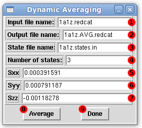
The Dynamic Averaging window allows the averaging of RDC data over dynamic domains of a structure. Only equations that correspond to the mobile domain should be selected when performing dynamic averaging. A REDCAT input file is specified (1) that is identical to the currently loaded REDCAT file. A name for the output file is given in the "Output file name" entry box (2). The states file is provided (3) and the number of states is specified (4). The principal order parameters are give in the "Sxx" (5), "Syy" (6), and "Szz" (7) entry boxes. The principal order parameters are automatically populated by selecting a solution from the Message window. Clicking the "Average" button (8) creates the Dynamic Average REDCAT file named above (2) as well as modifying the RDC section of the selected equations. The "Done" button (9) hides the window. For more information, please refer to Tutorial 3 as well as the Dynamic Averaging File Format section of this website.

