


REDCAT Documentation Table of Contents
Viewing and Interpreting Results
Several windows are used in order to view and interpret results. After loading a REDCAT file and clicking the Run button on the Main window, the "Message!" window will appear. On this window the user is presented with some important information. The first column of data is the equation number. The equation number corresponds to the line labeled on the Main window. The next column of data is the number of rejections of Monte Carlo samples the equation contributed to. The last column of data is the error value. For more information on the Monte Carlo Sampling feature, please refer to the Monte Carlo Sampling section of this website.
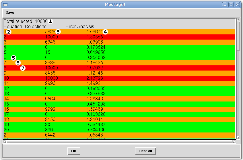
The total number of Monte Carlo rejections will be displayed first (1). In the case pictured above, 10,000 Monte Carlo samples were taken and out of those at least one equation contributed to the rejection of all 10,000 samples. If this number is less than the total number of Monte Carlo Samples taken, then when solutions are printed, there will be more than just the least squares solution present. In the next line of output, three columns are presented: the equation number (2), the number of rejections of Monte Carlo samples for that equation (3), and the error in Hz for that equation (4). To help with analysis, color coding is used to allow the user to quickly interpret results. If the equation line is green (5), then the number of rejections of Monte Carlos samples that the equation contributes to is below the total number of samples taken, and the error for the equation is less than the error specified for that equation on the Main window. If the line is orange (6), then the number of rejections of Monte Carlo samples the equation contributes to is less than the total number of samples taken, but the error for that equation is beyond the error specified for that equation on the Main window. If the line is red (7), then the equation contributes to the rejection of all Monte Carlo samples, and the error for the equation is beyond the error specified for that equation on the Main window. A fourth color, yellow (not pictured), is also used which describes the case where the equation contributed to the rejection of all Monte Carlo samples, but the error for the equation is below the error specified on the Main window for that equation. The table below summarizes the REDCAT color coding scheme and its relationship with the equations contribution to the Monte Carlo sample rejection and the equation's error.
| REDCAT Color Coding Scheme | ||
|---|---|---|
| Does Not Contribute to All Monte Carlo Rejections | Contributes to All Monte Carlo Rejections | |
| Is Below Error | ||
| Is Beyond Error | ||
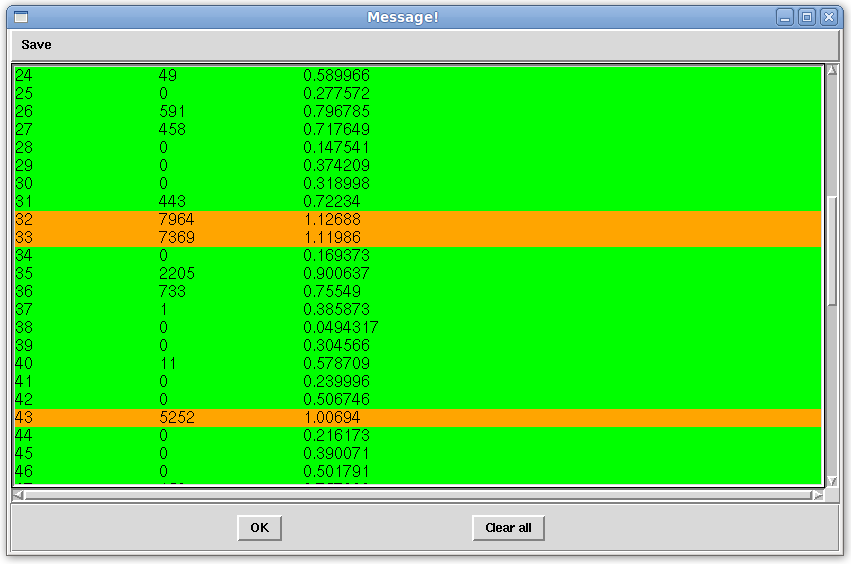
Following REDCAT's analusis of the data provided in the 1a1z.redcat file, the "Message!" window pictured above is obtained. Here, there are no red or yellow analysis lines, meaning that no equation contributes to rejection of all Monte Carlo samples. Thus, we have multiple Monte Carlo order tensor solutions to choose from.
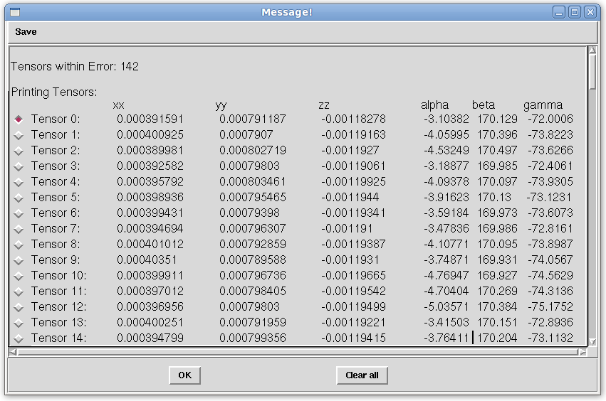
Once solutions are obtained they are appended to the "Message!" window, as pictured above, with Tensors 0-142. Selecting Tensor 0, the least squares solution, will load the principal order parameters and corresponding Euler rotations into the internal variables of REDCAT. These will then be used to back-calculate RDC data points, as demonstrated in the next step.
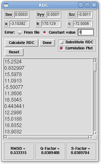
The RDC window, pictured above, is populated with the principal order parameters and Euler rotations selected from the "Message!" window. In the example above, RDCs are calculated with no noise by selecting the "Constant value" checkbox and typing a 0 in the entry box next to it. In order to see the plot of the loaded RDCs (Measured) to the back-calculated RDCs (Computed), the "Correlation Plot" checkbox is selected. By clicking the "Calculate RDC" button, the RDCs, RMSD, Q-Factor, and S-Factor are then computed. In the current example, the RMSD is roughly 0.53 Hz which is below experimental error specified of 1 Hz. Both the Q-Factor and S-Factor are also at around 3.8% which means that the computed and measured noise is very small, respectively. We can be sure that the data fits the structure well, and that the noise associated with the computed and measured RDCs is minor. Therefor, the data seems to be of good quality and the structure shows good fitness to the data.

Because we selected the "Correlation Plot" checkbox in the RDC window, a plot of the Computed (back-calculated) RDCs to Measured (loaded) RDCs is generated. An R2 regression line is fit to the data and in the above example it is very close to 45°, revealing that the computed and measured RDCs have good correlation.
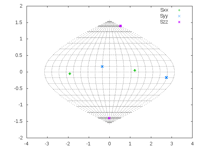
Next, we plot the order tensor on a Sanson-Flamsteed projection, as seen above. Using the 2D SF Plot window, we plot the order tensor. When the structure is in its principal alignment frame (PAF) - that is, when each Euler rotation is zero - the Sxx and Syy values fall on a strait line on the x-axis at 0, and the Szz values are at the very top and bottom of the projection. Utilizing this plot, the user may get an idea as to how the order tensor of the molecular frame may be rotated with respect to the PAF.
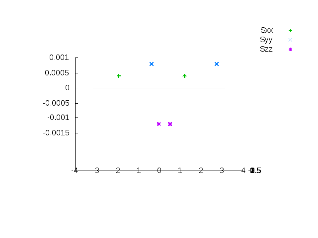
Using the values of the principal order parameters, the same SF plot may be generated in 3 dimensions, as pictured above. When the structure is in the PAF, the Szz values overlap and appear as one. This type of plot also provides more information related to how the molecular frame may be shifted.

